6 Claims reserving

6.1 Goals

You’ll focus on reserving analytics with run-off triangles, including the following steps:

importing a run-off triangle
visualizing the data in the triangle
basic chain-ladder calculations: the Mack approach
setting up a bootstrap analysis to simulate from the predictive distribution of the outstanding loss amount while incorporating parameter and process uncertainty.

6.2 Import a run-off triangle

6.2.1 Using `scan`

You can load a run-off triangle in many different ways. Here is a first strategy, using the scan() function in R.

Xij <- scan(n=55)
357848 766940 610542 482940 527326 574398 146342 139950 227229 67948
352118 884021 933894 1183289 445745 320996 527804 266172 425046
290507 1001799 926219 1016654 750816 146923 495992 280405
310608 1108250 776189 1562400 272482 352053 206286
443160 693190 991983 769488 504851 470639
396132 937085 847498 805037 705960
440832 847631 1131398 1063269
359480 1061648 1443370
376686 986608
344014

Exercise:

verify the structure of object Xij. What happened?

You will now reshape the flat vector Xij into a data frame that can be used for claims reserving with GLMs.

n <- length(Xij)
TT <- trunc(sqrt(2*n))
# row.nrs
i <- rep(1:TT, TT:1)
# col.nrs
j <- sequence(TT:1)
# calendar.nrs
c <- i+j-1
# as.factor
i <- as.factor(i)
j <- as.factor(j)
c <- as.factor(c)
# combine into a data frame
my_triangle_data <- data.frame(Xij, i, j, c)

Exercise:

verify the structure of the resulting data frame
inspect the first 10 rows using head.

You now prepare some first visual inspections of the data stored in my_triangle_data.

par(mfrow = c(2, 2))
boxplot(Xij ~ i, col = "grey", main = "Boxplot of payments vs AY")
boxplot(Xij ~ j, col = "grey", main = "Boxplot of payments vs DY")
boxplot(Xij ~ c, col = "grey", main = "Boxplot of payments vs CY")
par(mfrow = c(1, 1))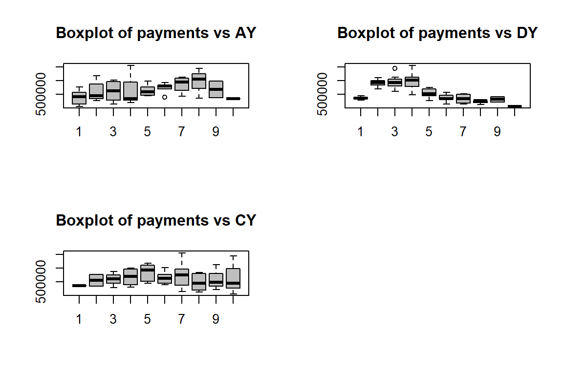

6.2.2 Using the `chainladder` package

The ChainLadder package is a well-developed and highly useful package for claims reserving in R. Among others the package brings functions covering:

Mack chain-ladder, Munich chain-ladder and bootstrap models
General multivariate chain ladder-models
Loss development factor fitting and Cape Cod models
Generalized linear models
One year claims development result functions
Utility functions to:

convert tables into triangles and triangles into tables
convert cumulative into incremental and incremental into cumulative triangles
visualise triangles.

You’ll now load the triangle introduced above with the ChainLadder package. Here is how this works.

path <- file.path("C:/Users/u0043788/Dropbox/Risk modelling course Ljubljana/Bookdown/data")
path.triangle <- file.path(path, "TaylorAshe.txt")
my_triangle_data_set <- read.table(path.triangle, header = TRUE, sep="\t")

Using the as.triangle function from the ChainLadder package you can reshape the data frame into a ‘triangle’.

#install.packages("ChainLadder")
library(ChainLadder)
# prepare triangle
my_triangle <- as.triangle(my_triangle_data_set, origin = "NumAY", dev = "NumDY", value = "Paym")
my_triangle

     NumDY
NumAY      1       2       3       4      5      6      7      8      9    10
   1  357848  766940  610542  482940 527326 574398 146342 139950 227229 67948
   2  352118  884021  933894 1183289 445745 320996 527804 266172 425046    NA
   3  290507 1001799  926219 1016654 750816 146923 495992 280405     NA    NA
   4  310608 1108250  776189 1562400 272482 352053 206286     NA     NA    NA
   5  443160  693190  991983  769488 504851 470639     NA     NA     NA    NA
   6  396132  937085  847498  805037 705960     NA     NA     NA     NA    NA
   7  440832  847631 1131398 1063269     NA     NA     NA     NA     NA    NA
   8  359480 1061648 1443370      NA     NA     NA     NA     NA     NA    NA
   9  376686  986608      NA      NA     NA     NA     NA     NA     NA    NA
   10 344014      NA      NA      NA     NA     NA     NA     NA     NA    NA

Exercise:

interpret the arguments of the function as.triangle
what is the structure of the R object my_triangle?

Here is an illustration of some useful functions from the package. Can you figure out what they do?

my_triangle_cum <- incr2cum(my_triangle)
my_triangle_cum

     NumDY
NumAY      1       2       3       4       5       6       7       8       9
   1  357848 1124788 1735330 2218270 2745596 3319994 3466336 3606286 3833515
   2  352118 1236139 2170033 3353322 3799067 4120063 4647867 4914039 5339085
   3  290507 1292306 2218525 3235179 3985995 4132918 4628910 4909315      NA
   4  310608 1418858 2195047 3757447 4029929 4381982 4588268      NA      NA
   5  443160 1136350 2128333 2897821 3402672 3873311      NA      NA      NA
   6  396132 1333217 2180715 2985752 3691712      NA      NA      NA      NA
   7  440832 1288463 2419861 3483130      NA      NA      NA      NA      NA
   8  359480 1421128 2864498      NA      NA      NA      NA      NA      NA
   9  376686 1363294      NA      NA      NA      NA      NA      NA      NA
   10 344014      NA      NA      NA      NA      NA      NA      NA      NA
     NumDY
NumAY      10
   1  3901463
   2       NA
   3       NA
   4       NA
   5       NA
   6       NA
   7       NA
   8       NA
   9       NA
   10      NA

plot(my_triangle)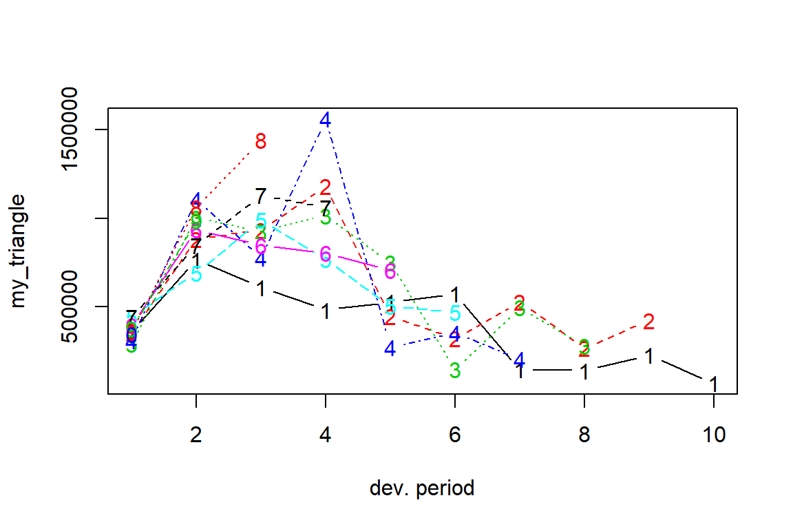

plot(my_triangle_cum)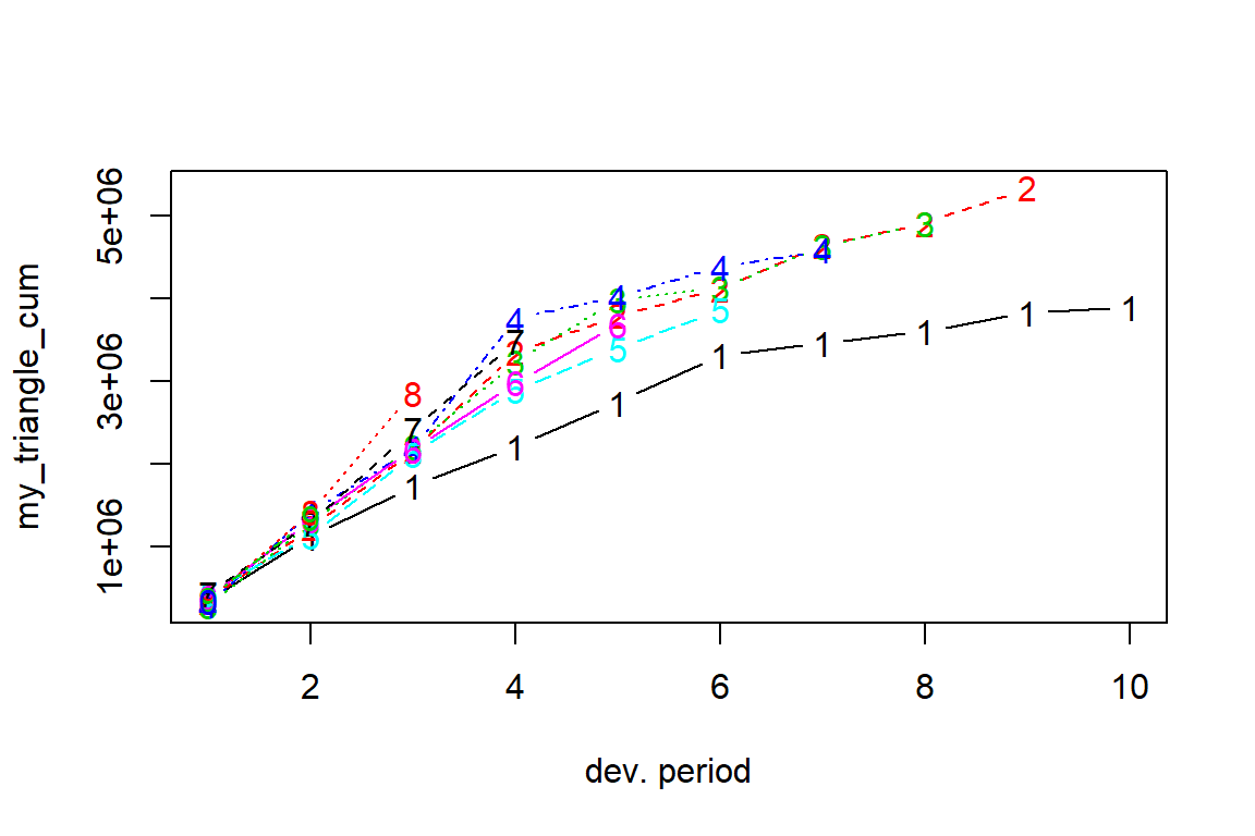

plot(my_triangle, lattice = TRUE)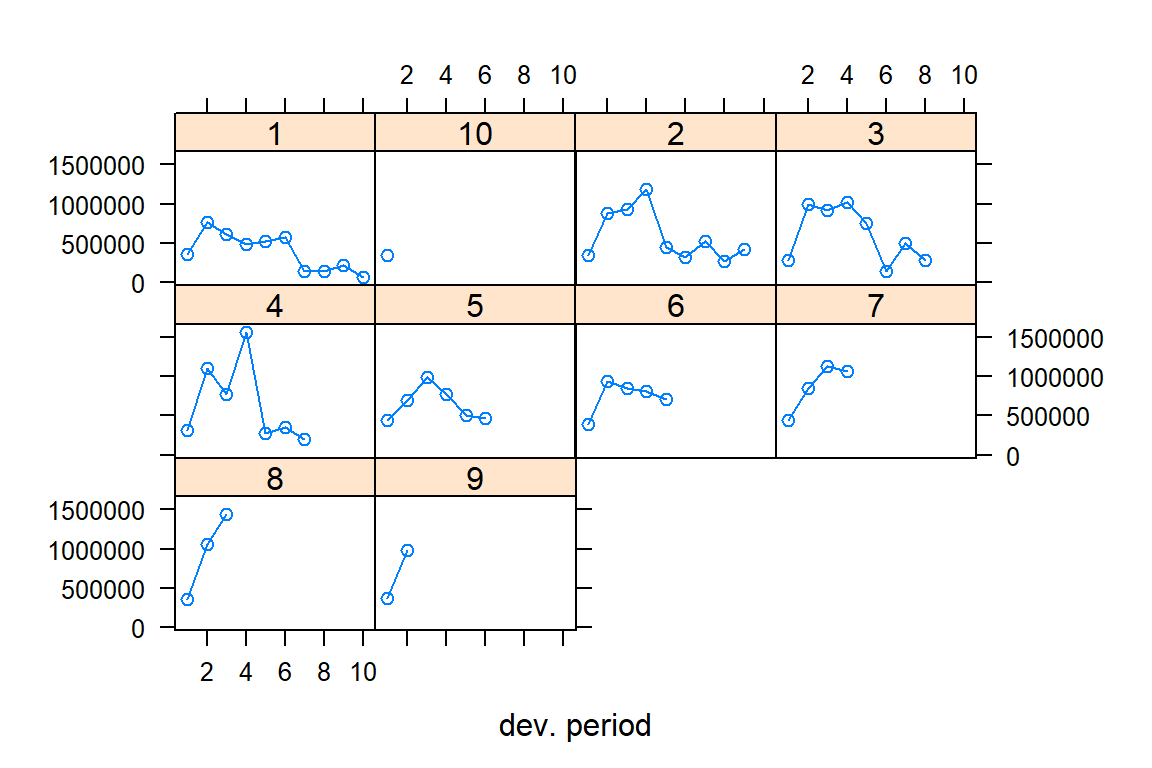

plot(my_triangle_cum, lattice = TRUE)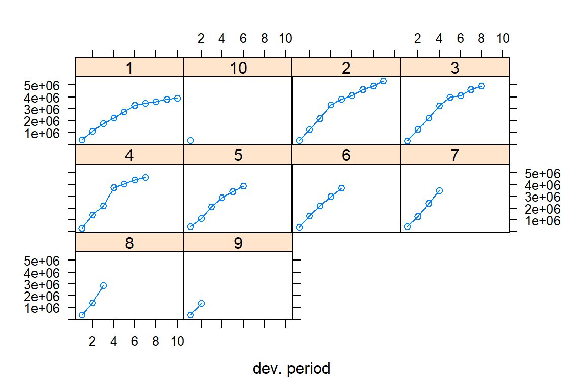

getLatestCumulative(my_triangle_cum)

      1       2       3       4       5       6       7       8       9      10 
3901463 5339085 4909315 4588268 3873311 3691712 3483130 2864498 1363294  344014 
attr(,"latestcol")
 1  2  3  4  5  6  7  8  9 10 
10  9  8  7  6  5  4  3  2  1 
attr(,"rowsname")
[1] "NumAY"
attr(,"colnames")
 [1] "10" "9"  "8"  "7"  "6"  "5"  "4"  "3"  "2"  "1" 
attr(,"colsname")
[1] "NumDY"

6.3 Mack’s Chain-Ladder calculations

The ChainLadder package can easily perform Mack’s calculations (see the lecture notes by Katrien for more details).

M <- MackChainLadder(my_triangle_cum, est.sigma = "Mack")
M

MackChainLadder(Triangle = my_triangle_cum, est.sigma = "Mack")

      Latest Dev.To.Date  Ultimate      IBNR  Mack.S.E CV(IBNR)
1  3,901,463      1.0000 3,901,463         0         0      NaN
2  5,339,085      0.9826 5,433,719    94,634    75,535    0.798
3  4,909,315      0.9127 5,378,826   469,511   121,699    0.259
4  4,588,268      0.8661 5,297,906   709,638   133,549    0.188
5  3,873,311      0.7973 4,858,200   984,889   261,406    0.265
6  3,691,712      0.7223 5,111,171 1,419,459   411,010    0.290
7  3,483,130      0.6153 5,660,771 2,177,641   558,317    0.256
8  2,864,498      0.4222 6,784,799 3,920,301   875,328    0.223
9  1,363,294      0.2416 5,642,266 4,278,972   971,258    0.227
10   344,014      0.0692 4,969,825 4,625,811 1,363,155    0.295

                 Totals
Latest:   34,358,090.00
Dev:               0.65
Ultimate: 53,038,945.61
IBNR:     18,680,855.61
Mack.S.E   2,447,094.86
CV(IBNR):          0.13

# get development factors
M$f

 [1] 3.491 1.747 1.457 1.174 1.104 1.086 1.054 1.077 1.018 1.000

# get the estimates for \sigma^2
M$sigma^2

[1] 160280.3  37736.9  41965.2  15182.9  13731.3   8185.8    446.6   1147.4
[9]    446.6

# get the full triangle
M$FullTriangle

      dev
origin      1       2       3       4       5       6       7       8       9
    1  357848 1124788 1735330 2218270 2745596 3319994 3466336 3606286 3833515
    2  352118 1236139 2170033 3353322 3799067 4120063 4647867 4914039 5339085
    3  290507 1292306 2218525 3235179 3985995 4132918 4628910 4909315 5285148
    4  310608 1418858 2195047 3757447 4029929 4381982 4588268 4835458 5205637
    5  443160 1136350 2128333 2897821 3402672 3873311 4207459 4434133 4773589
    6  396132 1333217 2180715 2985752 3691712 4074999 4426546 4665023 5022155
    7  440832 1288463 2419861 3483130 4088678 4513179 4902528 5166649 5562182
    8  359480 1421128 2864498 4174756 4900545 5409337 5875997 6192562 6666635
    9  376686 1363294 2382128 3471744 4075313 4498426 4886502 5149760 5544000
    10 344014 1200818 2098228 3057984 3589620 3962307 4304132 4536015 4883270
      dev
origin      10
    1  3901463
    2  5433719
    3  5378826
    4  5297906
    5  4858200
    6  5111171
    7  5660771
    8  6784799
    9  5642266
    10 4969825

# get Mack SE
M$Mack.S.E

      dev
origin 1      2      3      4      5       6       7       8       9      10
    1  0      0      0      0      0       0       0       0       0       0
    2  0      0      0      0      0       0       0       0       0   75535
    3  0      0      0      0      0       0       0       0   94225  121699
    4  0      0      0      0      0       0       0   52792  109210  133549
    5  0      0      0      0      0       0  198502  215088  247694  261406
    6  0      0      0      0      0  247204  337617  359530  397610  411010
    7  0      0      0      0 250737  381475  468091  496372  543209  558317
    8  0      0      0 378275 524309  648532  745376  787969  855493  875328
    9  0      0 241429 489488 626722  739750  832421  878987  951274  971258
    10 0 246656 486186 776148 940318 1066053 1175373 1239733 1337626 1363155

# split parameter and process risk
M$Mack.ProcessRisk

      dev
origin 1      2      3      4      5       6       7       8       9      10
    1  0      0      0      0      0       0       0       0       0       0
    2  0      0      0      0      0       0       0       0       0   48832
    3  0      0      0      0      0       0       0       0   75052   90524
    4  0      0      0      0      0       0       0   45268   89011  102622
    5  0      0      0      0      0       0  178062  192597  219267  227880
    6  0      0      0      0      0  225149  305242  324745  357179  366582
    7  0      0      0      0 229965  347244  423348  448603  489045  500202
    8  0      0      0 346712 478565  588507  673019  711125  770192  785741
    9  0      0 226818 457429 583978  686644  770169  813005  878614  895570
    10 0 234816 462237 736128 890565 1007785 1109441 1170034 1261670 1284882

M$Mack.ParameterRisk

      dev
origin 1     2      3      4      5      6      7      8      9     10
    1  0     0      0      0      0      0      0      0      0      0
    2  0     0      0      0      0      0      0      0      0  57628
    3  0     0      0      0      0      0      0      0  56970  81338
    4  0     0      0      0      0      0      0  27163  63275  85464
    5  0     0      0      0      0      0  87733  95756 115215 128078
    6  0     0      0      0      0 102068 144266 154280 174690 185867
    7  0     0      0      0  99925 157940 199712 212463 236456 248023
    8  0     0      0 151271 214185 272494 320359 339405 372388 385759
    9  0     0  82715 174234 227486 275226 315855 334127 364636 375893
    10 0 75503 150710 246013 301814 347618 388126 409829 444333 455270

sqrt(M$Mack.ProcessRisk^2+M$Mack.ParameterRisk^2)

      dev
origin 1      2      3      4      5       6       7       8       9      10
    1  0      0      0      0      0       0       0       0       0       0
    2  0      0      0      0      0       0       0       0       0   75535
    3  0      0      0      0      0       0       0       0   94225  121699
    4  0      0      0      0      0       0       0   52792  109210  133549
    5  0      0      0      0      0       0  198502  215088  247694  261406
    6  0      0      0      0      0  247204  337617  359530  397610  411010
    7  0      0      0      0 250737  381475  468091  496372  543209  558317
    8  0      0      0 378275 524309  648532  745376  787969  855493  875328
    9  0      0 241429 489488 626722  739750  832421  878987  951274  971258
    10 0 246656 486186 776148 940318 1066053 1175373 1239733 1337626 1363155

Again, the package can nicely visualize the results.

plot(M)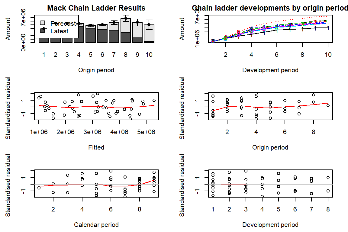

plot(M,lattice=TRUE)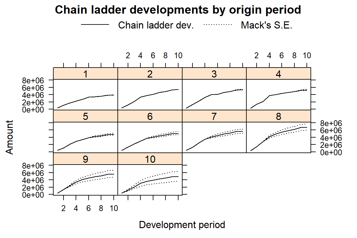

Exercise:

interpret the plots. What do you see?

6.4 GLM analysis of a run-off triangle

Next to Mack’s chain ladder calculation, you can also work with the data frame my_triangle_data and build a (overdispersed) Poisson GLM for these data.

str(my_triangle_data)

'data.frame':   55 obs. of  4 variables:
 $ Xij: num  357848 766940 610542 482940 527326 ...
 $ i  : Factor w/ 10 levels "1","2","3","4",..: 1 1 1 1 1 1 1 1 1 1 ...
 $ j  : Factor w/ 10 levels "1","2","3","4",..: 1 2 3 4 5 6 7 8 9 10 ...
 $ c  : Factor w/ 10 levels "1","2","3","4",..: 1 2 3 4 5 6 7 8 9 10 ...

# Poisson GLM of Xij versus i+j
poi_glm <- glm(Xij ~ i + j, poisson(link=log), data = my_triangle_data)
summary(poi_glm)


Call:
glm(formula = Xij ~ i + j, family = poisson(link = log), data = my_triangle_data)

Deviance Residuals: 
   Min      1Q  Median      3Q     Max  
-464.9  -123.7   -21.7   116.2   494.3  

Coefficients:
             Estimate Std. Error  z value Pr(>|z|)    
(Intercept) 12.506405   0.000754 16587.37  < 2e-16 ***
i2           0.331272   0.000669   494.85  < 2e-16 ***
i3           0.321119   0.000688   466.96  < 2e-16 ***
i4           0.305960   0.000701   436.57  < 2e-16 ***
i5           0.219316   0.000732   299.46  < 2e-16 ***
i6           0.270077   0.000745   362.76  < 2e-16 ***
i7           0.372208   0.000761   489.34  < 2e-16 ***
i8           0.553333   0.000813   680.38  < 2e-16 ***
i9           0.368934   0.001043   353.77  < 2e-16 ***
i10          0.242033   0.001864   129.83  < 2e-16 ***
j2           0.912526   0.000649  1406.04  < 2e-16 ***
j3           0.958831   0.000665  1441.37  < 2e-16 ***
j4           1.025997   0.000684  1499.93  < 2e-16 ***
j5           0.435276   0.000802   542.81  < 2e-16 ***
j6           0.080057   0.000936    85.49  < 2e-16 ***
j7          -0.006381   0.001039    -6.14  8.1e-10 ***
j8          -0.394452   0.001353  -291.56  < 2e-16 ***
j9           0.009378   0.001396     6.72  1.9e-11 ***
j10         -1.379907   0.003910  -352.95  < 2e-16 ***
---
Signif. codes:  0 '***' 0.001 '**' 0.01 '*' 0.05 '.' 0.1 ' ' 1

(Dispersion parameter for poisson family taken to be 1)

    Null deviance: 10699464  on 54  degrees of freedom
Residual deviance:  1903014  on 36  degrees of freedom
AIC: 1903877

Number of Fisher Scoring iterations: 4

# get coefficients of this regression model
coef(poi_glm)

(Intercept)          i2          i3          i4          i5          i6 
  12.506405    0.331272    0.321119    0.305960    0.219316    0.270077 
         i7          i8          i9         i10          j2          j3 
   0.372208    0.553333    0.368934    0.242033    0.912526    0.958831 
         j4          j5          j6          j7          j8          j9 
   1.025997    0.435276    0.080057   -0.006381   -0.394452    0.009378 
        j10 
  -1.379907

Exercise:

write down the full model specification of this GLM.

Using the coefficients stored in poi_glm you want to extract fitted values for upper and lower triangle.

# apply inverse link function
coefs <- exp(as.numeric(coef(poi_glm)))
alpha <- c(1, coefs[2:TT])*coefs[1]
alpha

 [1] 270061 376125 372325 366724 336287 353798 391842 469648 390561 344014

length(alpha)

[1] 10

beta  <- c(1, coefs[(TT+1):(2*TT-1)])
beta

 [1] 1.0000 2.4906 2.6086 2.7899 1.5454 1.0833 0.9936 0.6740 1.0094 0.2516

length(beta)

[1] 10

# fitted values, original scale
orig_fits <- alpha %*% t(beta)
dim(orig_fits)

[1] 10 10

str(orig_fits)

 num [1:10, 1:10] 270061 376125 372325 366724 336287 ...

orig_fits

        [,1]    [,2]    [,3]    [,4]   [,5]   [,6]   [,7]   [,8]   [,9]  [,10]
 [1,] 270061  672617  704494  753438 417350 292571 268344 182035 272606  67948
 [2,] 376125  936779  981176 1049342 581260 407474 373732 253527 379669  94634
 [3,] 372325  927316  971264 1038741 575388 403358 369957 250966 375833  93678
 [4,] 366724  913365  956652 1023114 566731 397290 364391 247190 370179  92268
 [5,] 336287  837559  877254  938200 519695 364316 334148 226674 339456  84611
 [6,] 353798  881172  922933  987053 546756 383287 351548 238477 357132  89016
 [7,] 391842  975923 1022175 1093189 605548 424501 389349 264121 395534  98588
 [8,] 469648 1169707 1225143 1310258 725788 508792 466660 316566 474073 118164
 [9,] 390561  972733 1018834 1089616 603569 423113 388076 263257 394241  98266
[10,] 344014  856804  897410  959756 531636 372687 341826 231882 347255  86555

Of course, you can also extract fitted.values from the GLM stored in poi_glm. What is the difference with our own coded approach?

fitted.values(poi_glm)

      1       2       3       4       5       6       7       8       9      10 
 270061  672617  704494  753438  417350  292571  268344  182035  272606   67948 
     11      12      13      14      15      16      17      18      19      20 
 376125  936779  981176 1049342  581260  407474  373732  253527  379669  372325 
     21      22      23      24      25      26      27      28      29      30 
 927316  971264 1038741  575388  403358  369957  250966  366724  913365  956652 
     31      32      33      34      35      36      37      38      39      40 
1023114  566731  397290  364391  336287  837559  877254  938200  519695  364316 
     41      42      43      44      45      46      47      48      49      50 
 353798  881172  922933  987053  546756  391842  975923 1022175 1093189  469648 
     51      52      53      54      55 
1169707 1225143  390561  972733  344014

# extract future
future <- row(orig_fits) + col(orig_fits) - 1 > TT
future

       [,1]  [,2]  [,3]  [,4]  [,5]  [,6]  [,7]  [,8]  [,9] [,10]
 [1,] FALSE FALSE FALSE FALSE FALSE FALSE FALSE FALSE FALSE FALSE
 [2,] FALSE FALSE FALSE FALSE FALSE FALSE FALSE FALSE FALSE  TRUE
 [3,] FALSE FALSE FALSE FALSE FALSE FALSE FALSE FALSE  TRUE  TRUE
 [4,] FALSE FALSE FALSE FALSE FALSE FALSE FALSE  TRUE  TRUE  TRUE
 [5,] FALSE FALSE FALSE FALSE FALSE FALSE  TRUE  TRUE  TRUE  TRUE
 [6,] FALSE FALSE FALSE FALSE FALSE  TRUE  TRUE  TRUE  TRUE  TRUE
 [7,] FALSE FALSE FALSE FALSE  TRUE  TRUE  TRUE  TRUE  TRUE  TRUE
 [8,] FALSE FALSE FALSE  TRUE  TRUE  TRUE  TRUE  TRUE  TRUE  TRUE
 [9,] FALSE FALSE  TRUE  TRUE  TRUE  TRUE  TRUE  TRUE  TRUE  TRUE
[10,] FALSE  TRUE  TRUE  TRUE  TRUE  TRUE  TRUE  TRUE  TRUE  TRUE

To conclude, you calculate the point estimates of the reserves (in total and per row) as obtained from the poi_glm fit.

# compare reserves with CL reserves
orig_reserve_tot <- sum(orig_fits[future])
orig_reserve_row <- numeric(TT-1)
for(i in 2:TT){
  orig_reserve_row[i-1] <- sum(orig_fits[i, (TT-i+2):TT])
}
point_est_glm <- data.frame(2:TT, orig_reserve_row)
names(point_est_glm) <- c("row", "reserve")
orig_reserve_tot

[1] 18680856

point_est_glm

  row reserve
1   2   94634
2   3  469511
3   4  709638
4   5  984889
5   6 1419459
6   7 2177641
7   8 3920301
8   9 4278972
9  10 4625811

Exercise:

compare the point estimates with the results stored in object M. What do you conclude?
now redo the analysis, use family = quasipoisson to do overdispersed Poisson instead of regular Poisson regression.

6.5 Bootstrap analysis

Starting from the results of an overdispersed Poisson GLM you can now code a bootstrap analysis to simulate from the predictive distribution of the outstanding reserve. Here is the preparatory work.

# OD Poisson GLM of Xij versus i+j
poi_glm_od <- glm(Xij ~ i + j, quasipoisson(link=log), data = my_triangle_data)
summary(poi_glm_od)


Call:
glm(formula = Xij ~ i + j, family = quasipoisson(link = log), 
    data = my_triangle_data)

Deviance Residuals: 
   Min      1Q  Median      3Q     Max  
-464.9  -123.7   -21.7   116.2   494.3  

Coefficients:
            Estimate Std. Error t value Pr(>|t|)    
(Intercept) 12.50640    0.17292   72.32  < 2e-16 ***
i2           0.33127    0.15354    2.16   0.0377 *  
i3           0.32112    0.15772    2.04   0.0492 *  
i4           0.30596    0.16074    1.90   0.0650 .  
i5           0.21932    0.16797    1.31   0.1999    
i6           0.27008    0.17076    1.58   0.1225    
i7           0.37221    0.17445    2.13   0.0398 *  
i8           0.55333    0.18653    2.97   0.0053 ** 
i9           0.36893    0.23918    1.54   0.1317    
i10          0.24203    0.42756    0.57   0.5749    
j2           0.91253    0.14885    6.13  4.7e-07 ***
j3           0.95883    0.15257    6.28  2.9e-07 ***
j4           1.02600    0.15688    6.54  1.3e-07 ***
j5           0.43528    0.18391    2.37   0.0234 *  
j6           0.08006    0.21477    0.37   0.7115    
j7          -0.00638    0.23829   -0.03   0.9788    
j8          -0.39445    0.31029   -1.27   0.2118    
j9           0.00938    0.32025    0.03   0.9768    
j10         -1.37991    0.89669   -1.54   0.1326    
---
Signif. codes:  0 '***' 0.001 '**' 0.01 '*' 0.05 '.' 0.1 ' ' 1

(Dispersion parameter for quasipoisson family taken to be 52602)

    Null deviance: 10699464  on 54  degrees of freedom
Residual deviance:  1903014  on 36  degrees of freedom
AIC: NA

Number of Fisher Scoring iterations: 4

# extract Pearson residuals
Prs.resid <- (my_triangle_data$Xij - fitted(poi_glm_od))/sqrt(fitted(poi_glm_od))
# get estimate dispersion parameter
n

[1] 55

p <- 2*TT-1
p

[1] 19

phi.P <- sum(Prs.resid^2)/(n-p)
phi.P

[1] 52601

# adjust the residuals for bias in the same way as scale parameter
Adj.Prs.resid <- Prs.resid*sqrt(n/(n-p))

And here starts the bootstrap loop, see Katrien’s lecture notes for explanation and schematic overview.

# initialize the random number generator
set.seed(6345789)

# i and j as factor variables
i <- rep(1:TT, TT:1); i <- as.factor(i)
j <- sequence(TT:1); j <- as.factor(j)

# run the bootstrap loop many times, eg 10000 times
nBoot <- 10000
payments <- numeric(nBoot)

for(boots in 1:nBoot){  ## start of the bootstrap loop
    # Step 1: resample from the adjusted residuals, with replacement
    Ps.Xij <- sample(Adj.Prs.resid, n, replace=TRUE)
    # Step 2: using this set of residuals and the estimated values of \hat{\mu_{ij}}
    # create a new suitable pseudo-history
    Ps.Xij <- Ps.Xij*sqrt(fitted(poi_glm_od))+fitted(poi_glm_od)
    Ps.Xij <- pmax(Ps.Xij, 0) 
    # Step 3: from this history, estimate \alpha_i, beta_j
    Ps.CL <- glm(Ps.Xij ~ i + j, quasipoisson)
    coefs <- exp(as.numeric(coef(Ps.CL)))
    Ps.alpha <- c(1, coefs[2:TT])*coefs[1]
    Ps.beta <- c(1, coefs[(TT+1):(2*TT-1)])
    # Step 4: compute fitted values, use sum of future part as an estimate of the reserve
    Ps.fits <- Ps.alpha%*%t(Ps.beta)
    Ps.reserve <- sum(Ps.fits[future])
    # Step 5: 
    Ps.totpayments <- phi.P*rpois(1, Ps.reserve/phi.P)
    # Step 6:
    payments[boots] <- Ps.totpayments
}
min(payments)

[1] 7416792

max(payments)

[1] 31981628

You extract useful summaries from the results stored in payments as follows.

quantile(payments, c(0.5, 0.75, 0.9, 0.95, 0.99), na.rm = TRUE)

     50%      75%      90%      95%      99% 
18673483 20672335 22671187 23986221 26826694

mean(payments)

[1] 18848278

sd(payments)

[1] 2968997

And plots

d <- data.frame(payments)
library(ggplot2)
ggplot(data=d, aes(payments)) + 
  geom_histogram(col = "black", fill = "blue", alpha = 0.2) + theme_bw() +
  labs(title = "Histogram for Bootstrap Reserves", x="Reserves", y="Count")

`stat_bin()` using `bins = 30`. Pick better value with `binwidth`.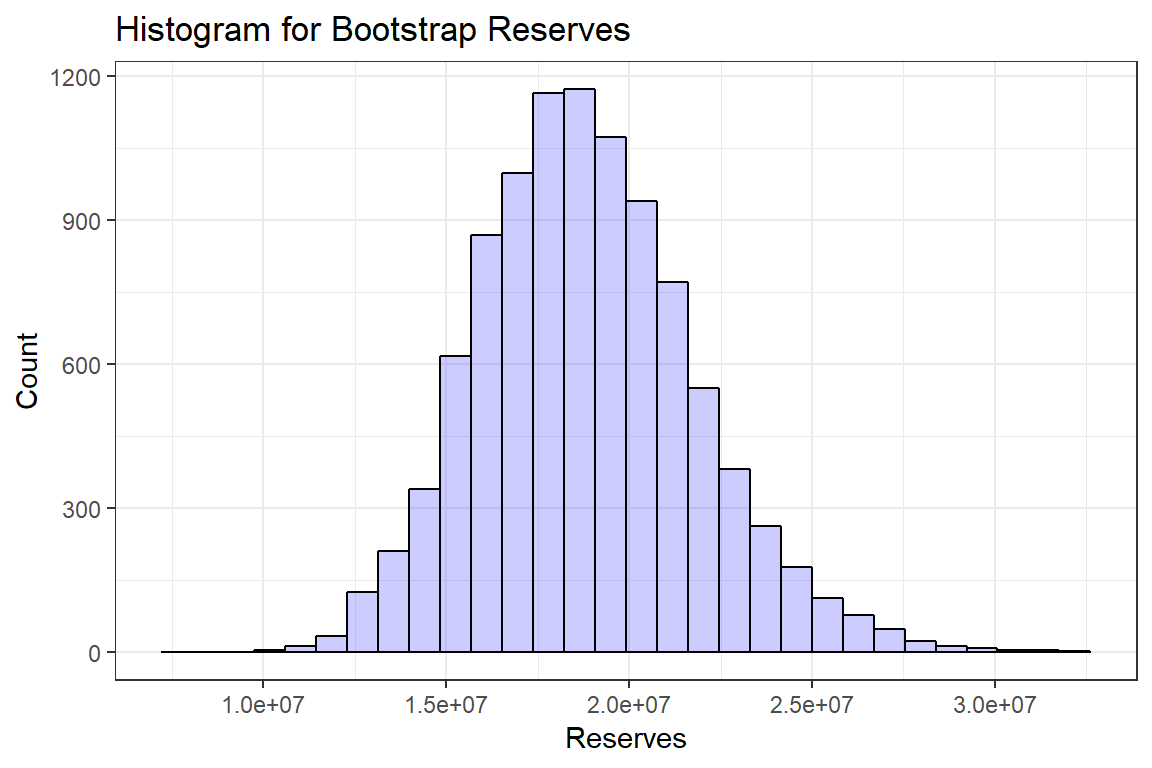

The ChainLadder package also has useful functions to set up bootstrap simulations.

set.seed(1)
B <- BootChainLadder(GenIns, R = 10000, process.distr = "od.pois")
B

BootChainLadder(Triangle = GenIns, R = 10000, process.distr = "od.pois")

      Latest Mean Ultimate Mean IBNR  IBNR.S.E  IBNR 75%  IBNR 95%
1  3,901,463     3,901,463         0         0         0         0
2  5,339,085     5,435,471    96,386   113,603   149,138   312,621
3  4,909,315     5,380,702   471,387   217,453   598,149   864,988
4  4,588,268     5,305,145   716,877   261,068   876,808 1,179,647
5  3,873,311     4,864,352   991,041   307,441 1,179,230 1,542,424
6  3,691,712     5,126,756 1,435,044   380,790 1,673,438 2,107,963
7  3,483,130     5,673,303 2,190,173   497,466 2,509,815 3,058,627
8  2,864,498     6,815,226 3,950,728   796,044 4,445,624 5,355,080
9  1,363,294     5,684,146 4,320,852 1,064,740 4,952,187 6,209,475
10   344,014     5,043,687 4,699,673 2,018,504 5,899,153 8,156,800

                    Totals
Latest:         34,358,090
Mean Ultimate:  53,230,252
Mean IBNR:      18,872,162
IBNR.S.E         3,001,662
Total IBNR 75%: 20,761,090
Total IBNR 95%: 24,064,106

plot(B)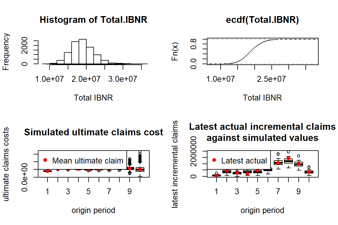

# some attributes o
B$Triangle

      dev
origin      1       2       3       4       5       6       7       8       9
    1  357848 1124788 1735330 2218270 2745596 3319994 3466336 3606286 3833515
    2  352118 1236139 2170033 3353322 3799067 4120063 4647867 4914039 5339085
    3  290507 1292306 2218525 3235179 3985995 4132918 4628910 4909315      NA
    4  310608 1418858 2195047 3757447 4029929 4381982 4588268      NA      NA
    5  443160 1136350 2128333 2897821 3402672 3873311      NA      NA      NA
    6  396132 1333217 2180715 2985752 3691712      NA      NA      NA      NA
    7  440832 1288463 2419861 3483130      NA      NA      NA      NA      NA
    8  359480 1421128 2864498      NA      NA      NA      NA      NA      NA
    9  376686 1363294      NA      NA      NA      NA      NA      NA      NA
    10 344014      NA      NA      NA      NA      NA      NA      NA      NA
      dev
origin      10
    1  3901463
    2       NA
    3       NA
    4       NA
    5       NA
    6       NA
    7       NA
    8       NA
    9       NA
    10      NA

B$f

 [1] 3.491 1.747 1.457 1.174 1.104 1.086 1.054 1.077 1.018 1.000

B$IBNR.Totals[1:10]

 [1] 21398909 17870368 17597508 18428981 19512320 19606687 15880725 22244763
 [9] 19325943 17354310

Risk Modelling in Insurance : a collection of computer labs in R

6 Claims reserving

6.1 Goals

6.2 Import a run-off triangle

6.2.1 Using `scan`

6.2.2 Using the `chainladder` package

6.3 Mack’s Chain-Ladder calculations

6.4 GLM analysis of a run-off triangle

6.5 Bootstrap analysis

6.6 More info

6 Claims reserving

6.1 Goals

6.2 Import a run-off triangle

6.2.1 Using scan

6.2.2 Using the chainladder package

6.3 Mack’s Chain-Ladder calculations

6.4 GLM analysis of a run-off triangle

6.5 Bootstrap analysis

6.6 More info

6.2.1 Using `scan`

6.2.2 Using the `chainladder` package