5 Generalized Linear Models
You’ll now study the use of Generalized Linear Models in R for insurance ratemaking. You focus first on the example from Rob Kaas’ et al. (2008) Modern Actuarial Risk Theory book (see Section 9.5 in this book), with simulated claim frequency data.
5.1 Modelling count data with Poisson regression models
5.1.1 A first data set
This example uses artifical, simulated data. You consider data on claim frequencies, registered on 54 risk cells over a period of 7 years. n gives the number of claims, and expo the corresponding number of policies in a risk cell; each policy is followed over a period of 7 years and n is the number of claims reported over this total period.
n <- scan(n = 54)
1  8 10  8  5 11 14 12 11 10  5 12 13 12 15 13 12 24
12 11  6  8 16 19 28 11 14  4 12  8 18  3 17  6 11 18
12  3 10 18 10 13 12 31 16 16 13 14  8 19 20  9 23 27

expo <- scan(n = 54) * 7
10 22 30 11 15 20 25 25 23 28 19 22 19 21 19 16 18 29
25 18 20 13 26 21 27 14 16 11 23 26 29 13 26 13 17 27
20 18 20 29 27 24 23 26 18 25 17 29 11 24 16 11 22 29

n
expo
[1] 1 8 10 8 5 11 14 12 11 10 5 12 13 12 15 13 12 24 12 11 6 8 16 19 28
[26] 11 14 4 12 8 18 3 17 6 11 18 12 3 10 18 10 13 12 31 16 16 13 14 8 19
[51] 20 9 23 27 [1] 70 154 210 77 105 140 175 175 161 196 133 154 133 147 133 112 126 203 175
[20] 126 140 91 182 147 189 98 112 77 161 182 203 91 182 91 119 189 140 126
[39] 140 203 189 168 161 182 126 175 119 203 77 168 112 77 154 203The goal is to illustrate ratemaking by explaining the expected number of claims as a function of a set of observable risk factors. Since artificial data are used in this example, you use simulated or self constructed risk factors. 4 factor variables are created, the sex of the policyholder (1=female and 2=male), the region where she lives (1=countryside, 2=elsewhere and 3=big city), the type of car (1=small, 2=middle and 3=big) and job class of the insured (1=civil servant/actuary/…, 2=in-between and 3=dynamic drivers). You use the R instruction rep() to construct these risk factors. In total 54 risk cells are created in this way. Note that you use the R instruction as.factor() to specify the risk factors as factor (or: categorical) covariates.
sex <- as.factor(rep(1:2, each=27, len=54))
region <- as.factor(rep(1:3, each=9, len=54))
type <- as.factor(rep(1:3, each=3, len=54))
job <- as.factor(rep(1:3, each=1, len=54))
sex
[1] 1 1 1 1 1 1 1 1 1 1 1 1 1 1 1 1 1 1 1 1 1 1 1 1 1 1 1 2 2 2 2 2 2 2 2 2 2 2
[39] 2 2 2 2 2 2 2 2 2 2 2 2 2 2 2 2
Levels: 1 2region [1] 1 1 1 1 1 1 1 1 1 2 2 2 2 2 2 2 2 2 3 3 3 3 3 3 3 3 3 1 1 1 1 1 1 1 1 1 2 2
[39] 2 2 2 2 2 2 2 3 3 3 3 3 3 3 3 3
Levels: 1 2 3type [1] 1 1 1 2 2 2 3 3 3 1 1 1 2 2 2 3 3 3 1 1 1 2 2 2 3 3 3 1 1 1 2 2 2 3 3 3 1 1
[39] 1 2 2 2 3 3 3 1 1 1 2 2 2 3 3 3
Levels: 1 2 3job [1] 1 2 3 1 2 3 1 2 3 1 2 3 1 2 3 1 2 3 1 2 3 1 2 3 1 2 3 1 2 3 1 2 3 1 2 3 1 2
[39] 3 1 2 3 1 2 3 1 2 3 1 2 3 1 2 3
Levels: 1 2 35.1.2 Fit a Poisson GLM
The response variable \(N_i\) is the number of claims reported on risk cell i, hence it is reasonable to assume a Poisson distribution for this random variable. You fit the following Poisson GLM to the data
\[\begin{eqnarray*} N_i &\sim& \text{POI}(d_i \cdot \lambda_i) \end{eqnarray*}\]
where \(\lambda_i = \exp{(\boldsymbol{x}^{'}_i\boldsymbol{\beta})}\) and \(d_i\) is the exposure for risk cell \(i\). In R you use the instruction glm to fit a GLM. Covariates are listed with +, and the log of expo is used as an offset. Indeed,
\[\begin{eqnarray*} N_i &\sim& \text{POI}(d_i \cdot \lambda_i) \\ &= & \text{POI}(\exp{(\boldsymbol{x}^{'}_i \boldsymbol{\beta}+\log{(d_i)})}) \end{eqnarray*}\]
The R instruction to fit this GLM (with sex, region, type and job the factor variables that construct the linear predictor) then goes as follows
g1 <- glm(n ~ sex + region + type + job + offset(log(expo)), fam = poisson(link = log))where the argument fam= indicates the distribution from the exponential family that is assumed. In this case you work with the Poisson distribution with logarithmic link (which is the default link in R). All available distributions and their default link functions are listed here http://stat.ethz.ch/R-manual/R-patched/library/stats/html/family.html.
You store the results of the glm fit in the object g1. You consult this object with the summary instruction
summary(g1)
Call:
glm(formula = n ~ sex + region + type + job + offset(log(expo)),
    family = poisson(link = log))

Deviance Residuals:
    Min       1Q   Median       3Q      Max
-1.9278  -0.6303  -0.0215   0.5380   2.3000

Coefficients:
            Estimate Std. Error z value Pr(>|z|)
(Intercept)  -3.0996     0.1229  -25.21  < 2e-16 ***
sex2          0.1030     0.0763    1.35   0.1771
region2       0.2347     0.0992    2.36   0.0180 *
region3       0.4643     0.0965    4.81  1.5e-06 ***
type2         0.3946     0.1017    3.88   0.0001 ***
type3         0.5844     0.0971    6.02  1.8e-09 ***
job2         -0.0362     0.0970   -0.37   0.7091
job3          0.0607     0.0926    0.66   0.5121
---
Signif. codes:  0 '***' 0.001 '**' 0.01 '*' 0.05 '.' 0.1 ' ' 1

(Dispersion parameter for poisson family taken to be 1)

    Null deviance: 104.73  on 53  degrees of freedom
Residual deviance:  41.93  on 46  degrees of freedom
AIC: 288.2

Number of Fisher Scoring iterations: 4
This summary of a glm fit lists (among others) the following items:
- the covariates used in the model, the corresponding estimates for the regression parameters (\(\boldsymbol{\hat{\beta}}\)), their standard errors, \(z\) statistics and corresponding \(P\) values;
- the dispersion parameter used; for the standard Poisson regression model this dispersion parameter is equal to 1, as indicated in the
Routput; - the null deviance - the deviance of the model that uses only an intercept - and the residual deviance - the deviance of the current model;
- the null deviance corresponds to \(53\) degrees of freedom, that is \(54-1\) where \(54\) is the number of observations used and \(1\) the number of parameters (here: just the intercept);
- the residual deviance corresponds to \(54-8=46\) degrees of freedom, since it uses \(8\) parameters;
- the AIC calculated for the considered regression model;
- the number of Fisher’s iterations needed to get convergence of the iterative numerical method to calculate the MLEs of the regression parameters in \(\boldsymbol{\beta}\).
The instruction names shows the names of the variables stored within a glm object. One of these variables is called coef and contains the vector of regression parameter estimates (\(\hat{\boldsymbol{\beta}}\)). It can be extracted with the instruction g1$coef.
names(g1) [1] "coefficients" "residuals" "fitted.values"
[4] "effects" "R" "rank"
[7] "qr" "family" "linear.predictors"
[10] "deviance" "aic" "null.deviance"
[13] "iter" "weights" "prior.weights"
[16] "df.residual" "df.null" "y"
[19] "converged" "boundary" "model"
[22] "call" "formula" "terms"
[25] "data" "offset" "control"
[28] "method" "contrasts" "xlevels" g1$coef(Intercept) sex2 region2 region3 type2 type3
-3.09959 0.10303 0.23468 0.46434 0.39463 0.58443
job2 job3
-0.03617 0.06072 Other variables can be consulted in a similar way. For example, fitted values at the original level are \(\hat{\mu}_i=\exp{(\hat{\eta}_i)}\) where the fitted values at the level of the linear predictor are stored in \(\hat{\eta}_i=\log{(d_i)}+\boldsymbol{x}^{'}_i\hat{\boldsymbol{\beta}}\). You then plot the fitted values versus the observed number of claims n. You add two reference lines: the diagonal and the least squares line.
g1$fitted.values 1 2 3 4 5 6 7 8 9 10 11
3.155 6.694 10.057 5.149 6.772 9.948 14.149 13.646 13.832 11.170 7.310
12 13 14 15 16 17 18 19 20 21 22
9.326 11.247 11.989 11.951 11.450 12.424 22.053 12.548 8.713 10.667 9.682
23 24 25 26 27 28 29 30 31 32 33
18.676 16.619 24.311 12.158 15.308 3.847 7.758 9.662 15.049 6.506 14.336
34 35 36 37 38 39 40 41 42 43 44
8.156 10.286 17.999 8.844 7.677 9.398 19.029 17.087 16.734 18.246 19.893
45 46 47 48 49 50 51 52 53 54
15.173 13.909 9.122 17.145 9.081 19.110 14.036 10.979 21.179 30.758 g1$linear.predictors 1 2 3 4 5 6 7 8 9 10 11 12 13
1.149 1.901 2.308 1.639 1.913 2.297 2.650 2.613 2.627 2.413 1.989 2.233 2.420
14 15 16 17 18 19 20 21 22 23 24 25 26
2.484 2.481 2.438 2.520 3.093 2.530 2.165 2.367 2.270 2.927 2.811 3.191 2.498
27 28 29 30 31 32 33 34 35 36 37 38 39
2.728 1.347 2.049 2.268 2.711 1.873 2.663 2.099 2.331 2.890 2.180 2.038 2.240
40 41 42 43 44 45 46 47 48 49 50 51 52
2.946 2.838 2.817 2.904 2.990 2.720 2.633 2.211 2.842 2.206 2.950 2.642 2.396
53 54
3.053 3.426 plot(g1$fitted.values, n, xlab = "Fitted values", ylab = "Observed claims")
abline(lm(g1$fitted ~ n), col="light blue", lwd=2)
abline(0, 1, col = "dark blue", lwd=2)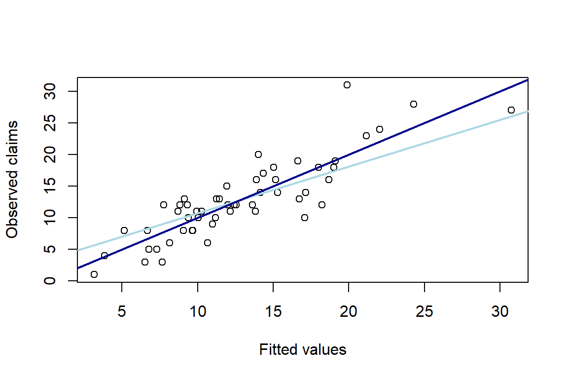
To extract the AIC you use
AIC(g1)[1] 288.25.1.3 The use of exposure
The use of expo, the exposure measure, in a Poisson GLM often leads to confusion. For example, the following glm instruction uses a transformed response variable \(n/expo\)
g2 <- glm(n/expo ~ sex+region+type+job,fam=poisson(link=log))
summary(g2)
Call:
glm(formula = n/expo ~ sex + region + type + job, family = poisson(link = log))

Deviance Residuals:
     Min        1Q    Median        3Q       Max
-0.16983  -0.05628  -0.00118   0.04680   0.17676

Coefficients:
            Estimate Std. Error z value Pr(>|z|)
(Intercept)  -3.1392     1.4846   -2.11    0.034 *
sex2          0.1007     0.9224    0.11    0.913
region2       0.2624     1.2143    0.22    0.829
region3       0.4874     1.1598    0.42    0.674
type2         0.4095     1.2298    0.33    0.739
type3         0.5757     1.1917    0.48    0.629
job2         -0.0308     1.1502   -0.03    0.979
job3          0.0957     1.1150    0.09    0.932
---
Signif. codes:  0 '***' 0.001 '**' 0.01 '*' 0.05 '.' 0.1 ' ' 1

(Dispersion parameter for poisson family taken to be 1)

    Null deviance: 0.77537  on 53  degrees of freedom
Residual deviance: 0.31739  on 46  degrees of freedom
AIC: Inf

Number of Fisher Scoring iterations: 5
and the object g3 stores the result of a Poisson fit on the same response variable, while taking expo into account as weights in the likelihood.
g3 <- glm(n/expo ~ sex+region+type+job,weights=expo,fam=poisson(link=log))
summary(g3)
Call:
glm(formula = n/expo ~ sex + region + type + job, family = poisson(link = log),
    weights = expo)

Deviance Residuals:
    Min       1Q   Median       3Q      Max
-1.9278  -0.6303  -0.0215   0.5380   2.3000

Coefficients:
            Estimate Std. Error z value Pr(>|z|)
(Intercept)  -3.0996     0.1229  -25.21  < 2e-16 ***
sex2          0.1030     0.0763    1.35   0.1771
region2       0.2347     0.0992    2.36   0.0180 *
region3       0.4643     0.0965    4.81  1.5e-06 ***
type2         0.3946     0.1017    3.88   0.0001 ***
type3         0.5844     0.0971    6.02  1.8e-09 ***
job2         -0.0362     0.0970   -0.37   0.7091
job3          0.0607     0.0926    0.66   0.5121
---
Signif. codes:  0 '***' 0.001 '**' 0.01 '*' 0.05 '.' 0.1 ' ' 1

(Dispersion parameter for poisson family taken to be 1)

    Null deviance: 104.73  on 53  degrees of freedom
Residual deviance:  41.93  on 46  degrees of freedom
AIC: Inf

Number of Fisher Scoring iterations: 5
Based on this output you conclude that g1 (with the log of exposure as offset in the linear predictor) and g3 are the same, but g2 is not. The mathematical explanation for this observation is given in the note ‘WeightsInGLMs.pdf’ available from Katrien’s lecture notes (available upon request).
5.1.4 Analysis of deviance for GLMs
5.1.4.1 The basics
You now focus on the selection of variables within a GLM based on a drop in deviance analysis. Your starting point is the GLM object g1 and the anova instruction.
g1 <- glm(n ~ 1 + region + type + job, poisson, offset = log(expo))
anova(g1, test="Chisq")
Analysis of Deviance Table
Model: poisson, link: log
Response: n
Terms added sequentially (first to last)
Df Deviance Resid. Df Resid. Dev Pr(>Chi)
NULL 53 104.7
region 2 21.6 51 83.1 2.0e-05 ***
type 2 38.2 49 44.9 5.1e-09 ***
job 2 1.2 47 43.8 0.55
---
Signif. codes: 0 '***' 0.001 '**' 0.01 '*' 0.05 '.' 0.1 ' ' 1The analysis of deviance table first summarizes the Poisson GLM object (response n, link is log, family is poisson). The table starts with the deviance of the NULL model (just using an intercept), and then adds risk factors sequentially. Recall that in this example only factor covariates are present. Adding region (which has three levels, and requires two dummy variables) to the NULL model causes a drop in deviance of 21.597, corresponding to 54-1-2 degrees of freedom and a resulting (residual) deviance of 83.135. The drop in deviance test allows to test whether the model term region is significant. That is:
\[ H_0: \beta_{\text{region}_2}=0\ \text{and}\ \beta_{\text{region}_3}=0. \]
The distribution of the corresponding test statistic is a Chi-squared distribution with 2 (i.e 53-51) degrees of freedom. The corresponding \(P\)-value is 2.043e-05. Hence, the model using region and the intercept is preferred above the NULL model. We can verify the \(P\)-value by calculating the following probability
\[ Pr(X > 21.597)\ \text{with}\ X \sim \chi^2_{2}.\]
Indeed, this is the probability - under \(H_0\) - to obtain a value of the test statistic that is the same or more extreme than the actual observed value of the test statistic. Calculations in R are as follows:
# p-value for region
1 - pchisq(21.597, 2)
[1] 2.043e-05# or
pchisq(21.597, 2, lower.tail = FALSE)[1] 2.043e-05Continuing the discussion of the above printed anova table, the next step is to add type to the model using an intercept and region. This causes a drop in deviance of 38.195. You conclude that also type is a significant model term. The last step adds job to the existing model (with intercept, region and type). You conclude that job does not have a significant impact when explaining the expected number of claims.
Based on this analysis of deviance table region and type seem to be relevant risk factors, but job is not, when explaining the expected number of claims.
The Chi-squared distribution is used here, since the regular Poisson regression model does not require the estimation of a dispersion parameter.
anova(g1,test="Chisq")The setting changes when the dispersion parameter is unknown and should be estimated. If you run the analysis of deviance for glm object g1 with the F distribution as distribution for the test statistic, you obtain:
# what if we use 'F' instead of 'Chisq'?
anova(g1,test="F")
Warning in anova.glm(g1, test = "F"): using F test with a 'poisson' family is
inappropriateAnalysis of Deviance Table
Model: poisson, link: log
Response: n
Terms added sequentially (first to last)
Df Deviance Resid. Df Resid. Dev F Pr(>F)
NULL 53 104.7
region 2 21.6 51 83.1 10.80 2.0e-05 ***
type 2 38.2 49 44.9 19.10 5.1e-09 ***
job 2 1.2 47 43.8 0.59 0.55
---
Signif. codes: 0 '***' 0.001 '**' 0.01 '*' 0.05 '.' 0.1 ' ' 1# not appropriate for regular Poisson regression, see Warning message in the console!and a Warning message is printed in the console that says
# Warning message:
# In anova.glm(g1, test = "F") :
#   using F test with a 'poisson' family is inappropriate
It is insightful to understand how the output shown for the \(F\) statistic and corresponding \(P\)-value is calculated. For example, the drop in deviance test comparing the NULL model viz a model using an intercept and region corresponds to an observed test statistic of 10.7985. The calculation of the \(F\) statistic requires
\[ \frac{\text{Drop-in-deviance}/q}{\hat{\phi}}, \]
where \(q\) is the difference in degrees of freedom between the compared models and \(\hat{\phi}\) is the estimate for the dispersion parameter. In this example \(F\) corresponding to region is calculated as
(21.597/2)/1[1] 10.8However, as explained, since the model investigated has a known dispersion, the Chi-squared test is most appropriate here. More details are here: https://stat.ethz.ch/R-manual/R-devel/library/stats/html/anova.glm.html.
5.1.5 An example
You are now ready to study a complete analysis-of-deviance table. This table investigates 10 possible model specifications g1-g10.
# construct an analysis-of-deviance table
g1 <- glm(n ~ 1, poisson , offset=log(expo))
g2 <- glm(n ~ sex, poisson , offset=log(expo))
g3 <- glm(n ~ sex+region, poisson, offset=log(expo))
g4 <- glm(n ~ sex+region+sex:region, poisson, offset=log(expo))
g5 <- glm(n ~ type, poisson, offset=log(expo))
g6 <- glm(n ~ region, poisson, offset=log(expo))
g7 <- glm(n ~ region+type, poisson, offset=log(expo))
g8 <- glm(n ~ region+type+region:type, poisson, offset=log(expo))
g9 <- glm(n ~ region+type+job, poisson, offset=log(expo))
g10 <- glm(n ~ region+type+sex, poisson, offset=log(expo))
For example, the residual deviance obtained with model g8 (using intercept, region, type and the interaction of region and type) is 42.4, see
summary(g8)
Call:
glm(formula = n ~ region + type + region:type, family = poisson,
    offset = log(expo))

Deviance Residuals:
    Min       1Q   Median       3Q      Max
-1.8296  -0.4893  -0.0622   0.5377   1.8974

Coefficients:
              Estimate Std. Error z value Pr(>|z|)
(Intercept)    -2.9887     0.1525  -19.60   <2e-16 ***
region2         0.1499     0.2061    0.73    0.467
region3         0.4216     0.1927    2.19    0.029 *
type2           0.4338     0.1985    2.19    0.029 *
type3           0.4520     0.1927    2.35    0.019 *
region2:type2  -0.0808     0.2664   -0.30    0.762
region3:type2  -0.0223     0.2537   -0.09    0.930
region2:type3   0.2556     0.2562    1.00    0.318
region3:type3   0.1086     0.2449    0.44    0.657
---
Signif. codes:  0 '***' 0.001 '**' 0.01 '*' 0.05 '.' 0.1 ' ' 1

(Dispersion parameter for poisson family taken to be 1)

    Null deviance: 104.732  on 53  degrees of freedom
Residual deviance:  42.412  on 45  degrees of freedom
AIC: 290.7

Number of Fisher Scoring iterations: 4g8$deviance[1] 42.41Using the technique of drop in deviance analysis you compare the models that are nested (!!) and decide which model specification is the preferred one. To do this, one can run multiple anova instructions such as
anova(g1, g2, test = "Chisq")Analysis of Deviance Table
Model 1: n ~ 1
Model 2: n ~ sex
Resid. Df Resid. Dev Df Deviance Pr(>Chi)
1 53 105
2 52 103 1 1.93 0.17which compares nested models g1 and g2, or g7 and g8
anova(g7, g8, test = "Chisq")Analysis of Deviance Table
Model 1: n ~ region + type
Model 2: n ~ region + type + region:type
Resid. Df Resid. Dev Df Deviance Pr(>Chi)
1 49 44.9
2 45 42.4 4 2.53 0.645.2 Overdispersed Poisson regression
The overdispersed Poisson model builds a regression model for the mean of the response variable
\[ EN_i = \exp{(\log d_i + \boldsymbol{x}_i^{'}\boldsymbol{\beta})} \]
and expressses the variance as
\[ \text{Var}(N_i) = \phi \cdot EN_i, \]
with \(N_i\) the number of claims reported by policyholder \(i\) and \(\phi\) an unknown dispersion parameter that should be estimated. This is called a quasi-Poisson model (see http://stat.ethz.ch/R-manual/R-patched/library/stats/html/family.html) and Section 1 in http://data.princeton.edu/wws509/notes/c4a.pdf for a more detailed explanation. To illustrate the differences between a regular Poisson and an overdispersed Poisson model, we fit the models g.poi and g.quasi:
g.poi <- glm(n ~ 1 + region + type, poisson, offset = log(expo))
summary(g.poi)
Call:
glm(formula = n ~ 1 + region + type, family = poisson, offset = log(expo))

Deviance Residuals:
    Min       1Q   Median       3Q      Max
-1.9233  -0.6564  -0.0573   0.4790   2.3144

Coefficients:
            Estimate Std. Error z value Pr(>|z|)
(Intercept)  -3.0313     0.1015  -29.86  < 2e-16 ***
region2       0.2314     0.0990    2.34   0.0195 *
region3       0.4605     0.0965    4.77  1.8e-06 ***
type2         0.3942     0.1015    3.88   0.0001 ***
type3         0.5833     0.0971    6.01  1.9e-09 ***
---
Signif. codes:  0 '***' 0.001 '**' 0.01 '*' 0.05 '.' 0.1 ' ' 1

(Dispersion parameter for poisson family taken to be 1)

    Null deviance: 104.73  on 53  degrees of freedom
Residual deviance:  44.94  on 49  degrees of freedom
AIC: 285.2

Number of Fisher Scoring iterations: 4
g.quasi <- glm(n ~ 1 + region + type, quasipoisson, offset = log(expo))
summary(g.quasi)
Call:
glm(formula = n ~ 1 + region + type, family = quasipoisson, offset = log(expo))

Deviance Residuals:
    Min       1Q   Median       3Q      Max
-1.9233  -0.6564  -0.0573   0.4790   2.3144

Coefficients:
            Estimate Std. Error t value Pr(>|t|)
(Intercept)  -3.0313     0.0961  -31.54  < 2e-16 ***
region2       0.2314     0.0938    2.47  0.01715 *
region3       0.4605     0.0913    5.04  6.7e-06 ***
type2         0.3942     0.0961    4.10  0.00015 ***
type3         0.5833     0.0919    6.35  6.8e-08 ***
---
Signif. codes:  0 '***' 0.001 '**' 0.01 '*' 0.05 '.' 0.1 ' ' 1

(Dispersion parameter for quasipoisson family taken to be 0.8965)

    Null deviance: 104.73  on 53  degrees of freedom
Residual deviance:  44.94  on 49  degrees of freedom
AIC: NA

Number of Fisher Scoring iterations: 4
Parameter estimates in both models are the same, but standard errors (and hence \(P\)-values) are not! You also see that g.poi reports z-value whereas g.quasi reports t-value, because the latter model estimates an extra parameter, i.e. the dispersion parameter.
Various methods are available to estimate the dispersion parameter, e.g.
\[ \hat{\phi} = \frac{\text{Deviance}}{n-(p+1)}\]
and
\[ \hat{\phi} = \frac{\text{Pearson}\ \chi^2}{n-(p+1)}\]
where \(p+1\) is the total number of parameters (including the intercept) used in the considered model. The (residual) deviance is the deviance of the considered model and can also be obtained as the sum of squared deviance residuals. The Pearson \(\chi^2\) statistic is the sum of the squared Pearson residuals. The latter is the default in R. Hence, you can verify the dispersion parameter of 0.896 as printed in the summary of g.quasi:
# dispersion parameter in g is estimated as follows
phi <- sum(residuals(g.poi, "pearson")^2)/g.poi$df.residual
phi
[1] 0.8965Since \(\hat{\phi}\) is less than 1, the result seems to indicate underdispersion. However, as discussed in Section 2.4 ‘Overdispersion’ in the book of Denuit et al. (2007), real data on reported claim counts very often reveal overdispersion. The counterintuitive result that is obtained here is probably due to the fact that artificial, self-constructed data are used.
When going from g.poi (regular Poisson) to g.quasi the standard errors are changed as follows:
\[ \text{SE}_{\text{Q-POI}} = \sqrt{\hat{\phi}} \cdot \text{SE}_{\text{POI}},\]
where \(\text{Q-POI}\) is for quasi-Poisson.
As a last step, you run the analysis of deviance for the quasi-Poisson model:
anova(g.quasi, test = "F")Analysis of Deviance Table
Model: quasipoisson, link: log
Response: n
Terms added sequentially (first to last)
Df Deviance Resid. Df Resid. Dev F Pr(>F)
NULL 53 104.7
region 2 21.6 51 83.1 12.0 5.6e-05 ***
type 2 38.2 49 44.9 21.3 2.2e-07 ***
---
Signif. codes: 0 '***' 0.001 '**' 0.01 '*' 0.05 '.' 0.1 ' ' 1For example, the \(F\)-statistic for region is calculated as
F <- (21.597/2)/phi
F
[1] 12.04and the corresponding \(P\)-value is
pf(F, 2, 49, lower.tail = FALSE)[1] 5.564e-055.3 Negative Binomial regression
You now focus on the use of yet another useful count regression model, that is the Negative Binomial regression model. The routine to fit a NB regression model is available in the package MASS and is called glm.nb, see https://stat.ethz.ch/R-manual/R-devel/library/MASS/html/glm.nb.html
# install.packages("MASS")
library(MASS)
g.nb <- glm.nb(n ~ 1+region+sex+offset(log(expo)))
summary(g.nb)
Call:
glm.nb(formula = n ~ 1 + region + sex + offset(log(expo)), init.theta = 26.38897379,
    link = log)

Deviance Residuals:
    Min       1Q   Median       3Q      Max
-2.6222  -0.6531  -0.0586   0.6587   2.3542

Coefficients:
            Estimate Std. Error z value Pr(>|z|)
(Intercept)  -2.7342     0.1019  -26.84  < 2e-16 ***
region2       0.2359     0.1195    1.97  0.04837 *
region3       0.4533     0.1176    3.85  0.00012 ***
sex2          0.1049     0.0939    1.12  0.26392
---
Signif. codes:  0 '***' 0.001 '**' 0.01 '*' 0.05 '.' 0.1 ' ' 1

(Dispersion parameter for Negative Binomial(26.39) family taken to be 1)

    Null deviance: 71.237  on 53  degrees of freedom
Residual deviance: 54.917  on 50  degrees of freedom
AIC: 316.1

Number of Fisher Scoring iterations: 1

              Theta:  26.4
          Std. Err.:  15.3

 2 x log-likelihood:  -306.1